Machine Learning
Pecas: Machine Learning Problem Shaping and Algorithm Selection

Introduction
In our previous article, Machine Learning Aided Time Tracking Review: A Business Case we introduced the business case behind Pecas, an internal tool designed to help us analyse and classify time tracking entries as valid or invalid.
This series will walk through the process of shaping the original problem as a machine learning problem and building the Pecas machine learning model and the Slackbot that makes its connection with Slack.
In this first article, we’ll talk through shaping the problem as a machine learning problem and gathering the data available to analyse and process.
Introduction
This series will consist of 6 posts focusing on the development of the Pecas machine learning model:
- Machine Learning Problem Shaping and Algorithm Selection <- You are here
- Data Preparation - Data Cleaning, Feature Engineering and Pre-processing
- Model Selection and Training - Training a Random Forest classifier
- Model Selection and Training - Training a Gradient Boosting classifier
- Model Evaluation - Cross-Validation and Fine-Tuning
- Model Deployment and Integration
Recap of the Business Problem
Before we dive into the machine learning aspect of the problem, let’s briefly recap the business problem that led to the solution being built.
OmbuLabs is a software development agency providing specialized services to a variety of different customers. Accurate time tracking is an important aspect of our business model, and a vital part of our work. Still, we faced several time tracking related issues over the years, related to accuracy, quality and timeliness of entries.
This came to a head at the end of 2022, when a report indicated we lost approximately one million dollars largely due to poor time tracking, which affected our invoicing and decision-making negatively. Up to this point, several different approaches had been taken to try to solve the problems, mostly related to different time tracking policies. All of these approaches ended up having significant flaws or negative side effects that led to policies being rolled back. This time, we decided to try to solve the problem differently.
There were a variety of time tracking issues, including time left unlogged, time logged to the wrong project, billable time logged as unbillable, incorrect time allocation, vague entries, among others. Measures put in place to try to mitigate the quality-related issues also led to extensive and time-consuming manual review processes, which were quite costly.
In other words, we needed to:
- Ensure the timeliness and quality of time entries;
- Do it with a process that wasn’t quite as costly (and therefore not scalable) as the existing manual process;
- Do it in a way that was fair to the team, and effective.
Our main idea was to replace (or largely replace) the manual process with an automated one. However, although the process was very repetitive, the complexity of the task (interpreting text) meant we needed a tool powerful enough to deal with that kind of data. Hence the idea to use machine learning to automate the time entry review process.
It is worth noting that machine learning powers one aspect of the solution: evaluating the quality and correctness of time entries. Other aspects such as timeliness of entries and completeness of the tracking for a given day or week are very easily solvable without a machine learning approach. Pecas is a combination of both, so it can be as effective as possible in solving the business problem as a whole.
Shaping the Machine Learning problem
The first thing we need to do is identify what part of the problem will be solved with the help of machine learning and how to properly frame that as a machine learning problem.
The component of the problem that is suitable for machine learning is the one that involves “checking” time entries for quality and accuracy, that is, the one that involves “interpreting” text. Ultimately, the goal is to understand if an entry meets the required standards or not and, if not, notify the team member who logged it to correct it.
Therefore, we have a classification problem in our hands. But what type of classification problem?
Our goal is to be able to classify entries according to pre-defined criteria. There are, in essence, two clear ways we can approach the classification:
- Final classification of the entry as valid or invalid
- Intermediate classification of the entry as belonging to a pre-defined category which is then checked against pre-defined criteria so validity or invalidity can be determined
Which one we want depends on a few different factors, perhaps the most important one being the existence of a finite, known number of ways in which an entry can be invalid.
If there is a finite, known number of classes an entry can belong to and a known number of ways in which each entry can be invalid, the machine learning model can be used to classify the entry as belonging to a specific category and that entry can then be checked against the specific criteria to determine validity or invalidity.
However, we don’t have that.
Time entries can belong to a wide range of categories as a mix of specific keywords in the description, project they’re logged to, tags applied to the entry, user who logged it, day the entry was logged, among many others. Too many. Therefore, intermediate classification might not be the best approach. Instead, we can use the entry’s characteristics to teach the model to identify entries that seem invalid, and let it determine validity or invalidity of the entry directly.
Thus we have in our hands a binary classification problem, whose objective is to classify time entries as valid or invalid.
Data Extraction and Initial Analysis
Now we know what kind of problem we have in our hands, but there are a wide variety of different algorithms that can help solve this problem. The decision of which one to use is best informed by the data itself. So let’s take a look at that.
The first thing we need is, of course, the time tracking data. We use Noko for time tracking, and it offers a friendly API for us to work with.
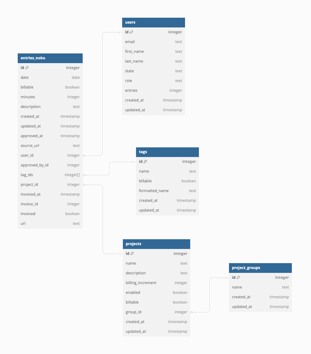
A Noko time entry as inputted by a user has a few different characteristics:
- A duration in minutes;
- A date the time tracked by the entry refers to;
- A project it is logged to;
- A description of the work performed;
- Tags that can be associated with it;
- A user who logged the entry.
There is also one relative characteristic of a time entry that is very important: whether it is billable or unbillable. This is
controlled by one of two entities: project or tag. Projects can be billable or unbillable. By default, all entries logged to an
unbillable project are unbillable and all entries logged to a billable project are billable. However, entries logged to a billable
project can be unbillable when a specific tag (the #unbillable tag) is added to the entry.
There is also some metadata and information that comes from user interaction with the system that can be associated with the entry, the most relevant ones being:
- A unique ID that identifies the entry in the system;
- The date the entry was created in the system (can be different from the date to which the entry refers);
- Whether the entry has been invoiced yet or not;
- Whether the entry has been approved by an admin user or not.
Of the entities associated with an entry, as mentioned above one is of particular interest: projects. As aforementioned, projects can indicate whether an entry is billable or unbillable. And, as you can imagine, an entry that belongs to a billable project logged to an unbillable project by mistake means the entry goes uninvoiced, and we lose money in the process.
A project also has a unique ID that identifies it, a name and a flag that indicates whether it is a billable or unbillable project. The flag and the ID are what matters to us for the classification, the ID because it allows us to link the project to the entry and the flag because it is the project characteristic we want to associate with the data.
There are other data sources that have relevant data that can be used to gain context on time entries, for example calendars, GitHub pull requests, Jira tickets. For now, let’s keep it simple, and use a dataset of time entries enriched with project data, all coming from Noko.
Initial Exploration
In order to make it easier to work and explore the data, we extracted all time entries from Noko logged between January 1st, 2022 and June 30th, 2023. In addition to entries, projects, tags and users were also extracted from Noko, and the data was loaded into a Postgres database, making it easy to explore with SQL.
We then extracted a few key characteristics from the set:
| property | stat |
|---|---|
| total_entries | 49451 |
| min_value | 0 |
| max_value | 720 |
| duration_q1 | 30 |
| duration_q3 | 90 |
| average_duration_iq | 49.39 |
| average_duration_overall | 71.33 |
| median_duration | 45 |
| max_word_count | 162 |
| min_word_count | 1 |
| avg_word_count | 9.89 |
| word_count_q1 | 4 |
| word_count_q3 | 11 |
| entries_in_word_count_iq | 29615 |
| average_word_count_iq | 6.63 |
| least_used_tag: ops-client | 1 |
| most_used_tag: calls | 12043 |
| unbillable_entries | 33987 |
| billable_entries | 15464 |
| pct_unbillable_entries | 68.73 |
| pct_billable_entries | 31.27 |
Data Interpretation
The table above allows us to get a good initial insight into the data and derive a few early conclusions:
- Data Size: For the problem at hand, our dataset is fairly large (over 49,000 entries), providing a substantial amount of data for analysis and training;
- Entry Duration: Duration values suggest a pretty wide range of time logged to an individual entry (varying between 0 and 720). Most entries tend towards short durations though (median of 45 minutes).
- Word Count: There’s significant variation in word count per entry (between 1 and 162), although it tends to be on the lower side (average of 9.89), indicating longer entries are the outlier.
- Tag Distribution: The number of least used tag indicates there are outliers in the data (tags only used once).
- Billable vs Unbillable Entries: The majority of entries are unbillable. The table does not include enough information to let us properly infer why.
This initial set of considerations already tells us something about our data. We have a fairly large dataset, with a mix of numerical and categorical variables. There are also outliers in several features of the data and the range of values in durations and word count could indicate their relationship with validity or invalidity is not strictly linear. Our empirical knowledge confirms this assumption. Although longer entries in duration are generally expected to have longer descriptions, there are several use cases for long entries in duration to have small word counts.
Other characteristics we looked at (in similar fashion) to get a good initial idea of what we were dealing with include:
- Number of entries per project;
- Most frequent duration per project;
- Number of entries per tag;
- Most frequent duration per tag;
- Occurrence of tags per project.
This gave us a good initial idea of what we were dealing with.
Algorithm Selection
By this point, we know we’re dealing with a binary classification problem and that we have a fairly large dataset with outliers and non-linear relationships in data. The dataset also has a mix of numerical and categorical variables. The problem we have at hand is made more complex by the presence of text data that requires interpretation.
There are a number of algorithms to choose from for binary classification, perhaps the most common being:
- Logistic Regression;
- K-Nearest Neighbors;
- Naive Bayes;
- Support Vector Machines;
- Tree-based models (such as Random Forest or Gradient Boosting).
A quick comparison of their strengths and weaknesses shows that tree-based models are most likely the right choice for our use case:
Logistic Regression
Logistic regression’s strengths lie in its simplicity:
- Coefficients of the model can be quite easily interpreted;
- Relatively low computational requirements, making it efficient.
However, some of its weaknesses make it clearly not a good candidate for our use case:
- Assumes a linear relationship between features and the log odds (logarithm, usually natural logarithm, of the odds of an event occurring) of the outcome;
- Might not perform well with complex, non-linear relationships in the data.
K-Nearest Neighbors
Another example of a simple algorithm, with strengths associated with its simplicity:
- It’s quite easy to understand and to implement;
- Works really well with small datasets.
However, some of its weaknesses also make it immediately not a good choice for our problem:
- Performs poorly on large datasets;
- The impact of irrelevant features or noise in the data is very significant.
Naive Bayes
Naive Bayes’ core strengths are:
- Fast training times, making it a good choice for baseline models;
- Performs quite well with smaller datasets and limited resources.
However, two key weaknesses make it yet another unsuitable choice for our use case:
- It assumes feature independence, which is not the case for us (and is quite rarely the case with any real-world data);
- Performs poorly with complex, non-linear relationships between features.
Support Vector Machine (SVM)
Unlike the previous algorithms, two of SVMs core strengths apply to our use case:
- It is effective in high-dimensional spaces;
- Allows flexibility in modeling various types of relationships.
However, two core weaknesses make it second to tree-based models as a choice:
- Training time on large datasets can be quite long;
- Requires careful tuning of hyperparameters.
Tree-based Models
We have arrived at the most suitable type of algorithm for our problem at hand! The core strengths of these algorithms that make them a good choice are:
- Good with mixed data types (numerical vs categorical variables);
- Can effectively capture complex, non-linear relationships in data;
- Tolerant to outliers and able to handle missing values in the set.
Some weaknesses related to them are:
- They can be computationally intensive, especially when using gradient boosting with a large dataset;
- Have a potential to overfit (learn too much about the training data and lose the ability to generalize), requiring careful tuning to avoid this.
Therefore, we’ll pick ensemble tree-based models as our starting point.
But which one? That’s a tale for the next post. We’ll do some more analysis in our data, pre-process it and train a few different models to pick the best one.
Conclusion
Framing your business problem (or business question) as a machine learning problem is a first and necessary step in understanding what kind of problem you’re dealing with and where to start solving it. It helps guide our data exploration and allows us to choose which machine learning algorithm (or family of algorithms) to start with.
A good understanding of the data available to you, the business context around the problem, and the characteristics that matter can help guide your exploration of the dataset to validate some initial questions, such as do we have enough data or is the data available enough to convey the information we need. It’s important to not be tied by these initial assumptions and this initial knowledge in your analysis though, as exploring the data might reveal additional, useful insights.
With a good understanding of the problem and dataset, you can make an informed algorithm selection, and start processing your data and engineering your features so your model can be trained. This second step is what we’ll look at in the next post.
Need help leveraging machine learning to solve complex business problems? Send us a message and let’s see how we can help!